In the previous post we talked about a series of geoprocesses related to criminology made together with Jaume I University (UJI). These geoprocesses can be used in different fields, not exclusively in criminology.

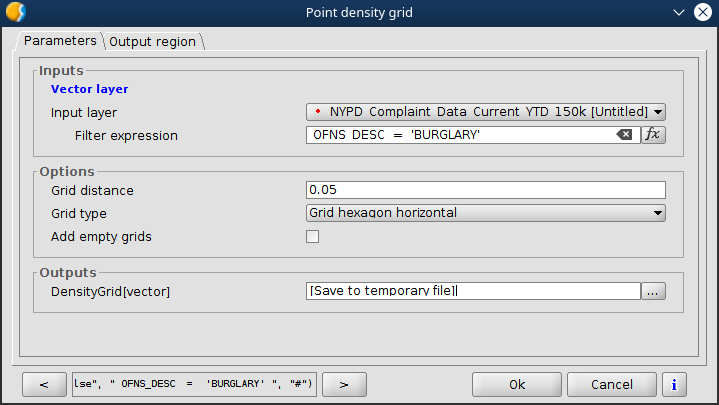
Now we are going to show the “Grid by point density” geoprocess. The main objective of this geoprocess is to perform a fast and efficient count of points contained in a grid, that also is created by the geoprocess. Here it has been raised for crimes, but it can be applied to many other things. It allows to visualize how events are distributed when there is a layer with a large accumulation of them in the same areas quickly.

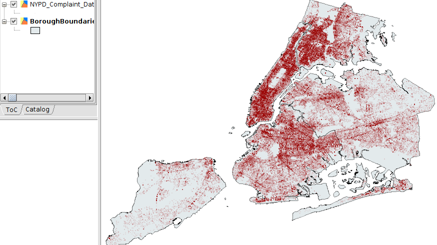
Crimes in New York (150.000 features)

The input parameters are a point layer and an expression (optional) that would be a filter to run the geoprocess. For example, we could apply a filter by type of crime.

The options make reference to:

• Grid distance: At the distance from the side of each square or hexagon. In relation to the measurements of the View.
• Grid type: It can be squared or hexagonal. And in hexagonal type there are two types: Vertical or horizontal.
• Add empty grids: It doesn’t add grid in areas where there are no specific elements, that is, where their count is zero.

It’s important to select the grid extension in the Analysis Region tab correctly.

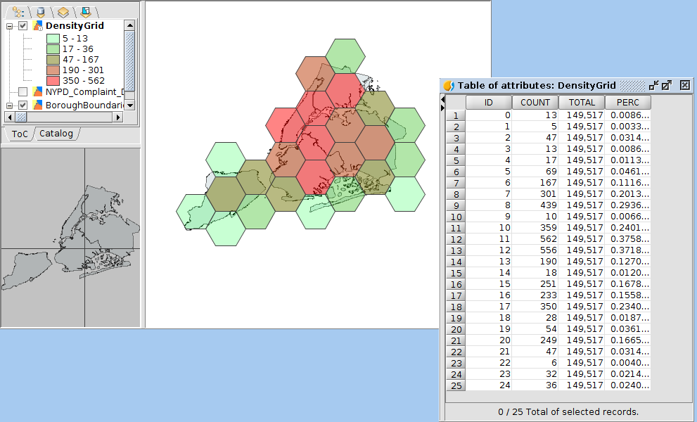
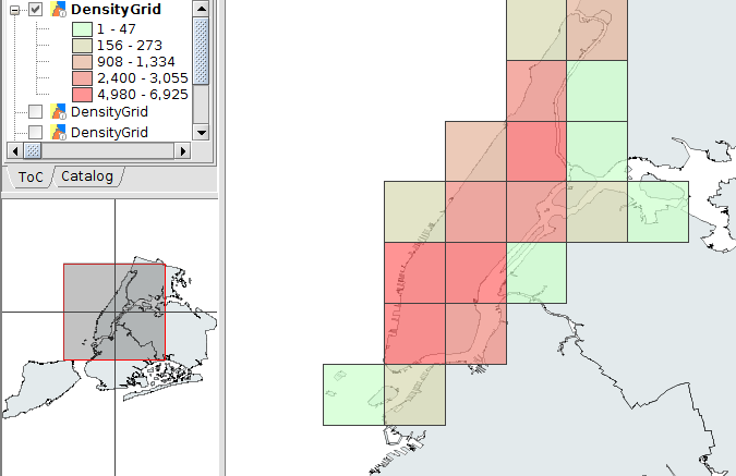
The results of the geoprocess on the starting image layer returns a grid with an attribute table, where we will be able to apply a legend by intervals of values.

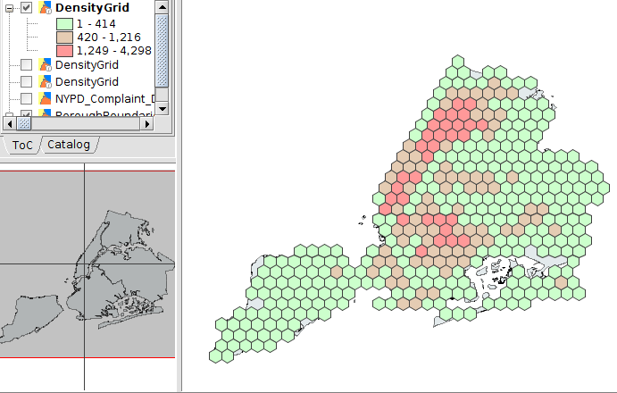
Here you can see the results on the complete crime layer with a shorter distance and vertical grid type.

And here applying a filter on a district.

In the attribute table you can see the total count of points within each grid, the total points involved in the initial calculation before filtering, and the percentage of those points in relation to the total.

In addition, we have taken advantage of this during the development of this geoprocess to improve and debug gvSIG to support layers with a larger number of records. One of these tests for this geoprocess was done with a layer with more than 6.7 million records and more than 10 fields.

You can now download and test the new Grid by point density geoprocess in the new distribution candidate to final version. You can download it from Tools -> Add-ons Manager, and search the “Geoprocess: Point density grid” geoprocess. Once installed and after restarting gvSIG, it will appear at the toolbox in the “Scripting – Data Analysis – Grid by density of points” section.

If you find any error or you have any recommendation, we encourage you to write to the gvSIG mailing lists.