In previous posts we spoke (Ring map and Grid by point density) about a series of geoprocesses related to criminology made together with Jaume I University (UJI). These geoprocesses can be used in different sectors, not exclusively related to criminology.

Now we are going to show the Aorist Clock geoprocess. The main objective of this geoprocess is to visualize the distribution of the temporal component in a graphical way. Its distribution within the hours of the same day, and within the day of the week will be shown.

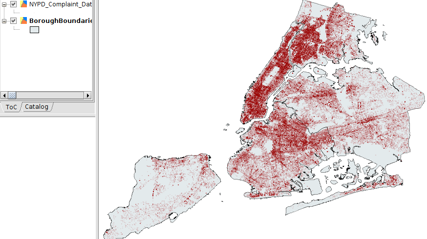
Crimes in New York (150.000 features)

This will generate a set of layers that will create a ring map representing the number of features located in each range of hours and days.

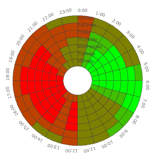
Example about the temporal distribution of the 150.000 crimes of New York

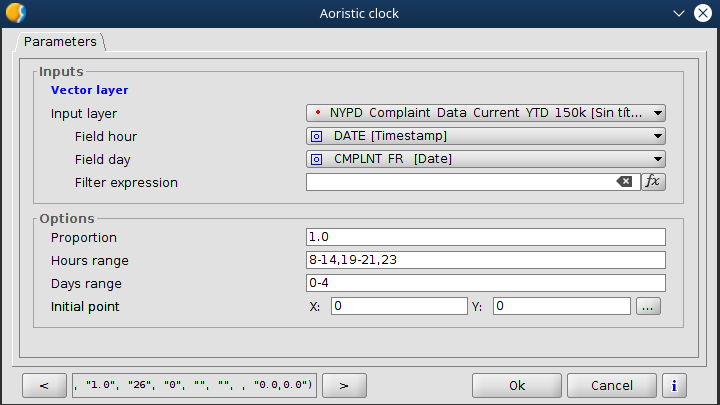
The input parameters are a layer with date fields that include the day of the week and the crime time. A filter could also be applied to analyze only a subset of data. For example, we could filter by type of crime.

The time type field has been generated by a calculated field to which the formula has been applied: TIMESTAMP (CMPLNT_F_1, ‘HH: mm: ss’), that converts a text type field similar to “03:15:00” in a Timestamp type field that supports hours, minutes and seconds values which are used in the geoprocess. This functionality will be explained in the next post about the new expression generator. You can ask any question about it at the mailing lists.

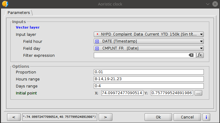
The geoprocess options are:

• Proportion: It allows you to modify the size of the ring map.
• Range of hours: It allows you to filter the range of hours to be analyzed. From 0 to 23.
• Range of days: It allows you to filter the range of days to analyze. From 0 to 6.
• Starting point: Placement of the ring map on the map.

These ranges can be established by writing the following text for the hours for example: 8-14,19-21,23. This means that it will analyze the hours in the range from 8 hours to 14 hours (from 8:00 to 14:59), from 19 to 21 hours, and also the 23 hours (which would include all events from 23:00 to 0:00)

These ranges allow to limit the temporal analysis. For example, looking at the first graph of all crimes, we see that they are mainly concentrated from midday to midnight, so an analysis of only that time slot will allow us to see their distribution in a better way.

To verify these ranges, we will run the geoprocess with the following parameters.

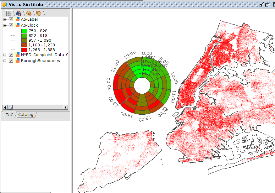
We will see a graph like this one:

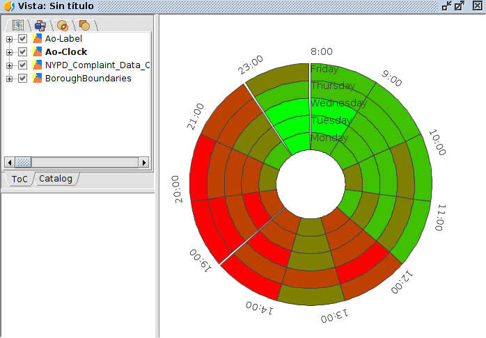
We can see that the graph has only be generated with the selected ranges. In the hour sectors where there is a temporal gap, the algorithm leaves a small blank space indicating that there is a discontinuity in that range.

The geoprocess generates several layers for the labels and for the ring. This allows you to modify everything related to your visualization, both labelling and legends.

In this case we are going to prepare it to appear in the New York area, giving us the possibility to print the map.

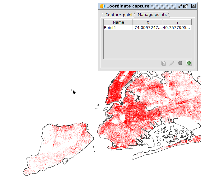
With the Coordinate Capture tool we will select a point close to the New York area.

Now we will run the geoprocess on that starting point. The proportion parameter is a function of the type of units of the view projection. In this case we have to reduce its size to a ratio of 0.01 to fit our map.

The results are these ones.

And if we created a map we would be able to have results similar to these ones.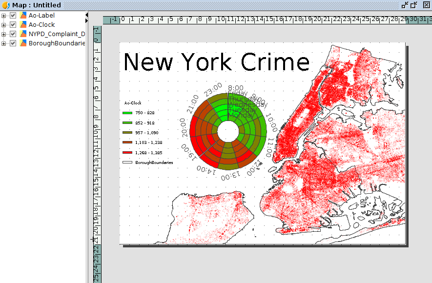In this example we have used a crime layer, but it could be used on any data set where a time field is available.

This geoprocess can be tested with the next Release Candidate version of gvSIG Desktop. You can download it from Tools -> Add-ons manager and search the “Geoprocess: Aoristic clock” geoprocess. Once installed, and after restarting gvSIG, it will appear at the “Scripting – Data Analysis – Aorist Clock” section.

If you have any doubt or you find any error you can send us the information through the mailing lists.