gvSIG 2.0: OpenStreetMap tiles

gvSIG 2.0 improves the raster access incorporating the possibility to make tiles for the sources of this type of data, local or remote ones. The results is that the raster layers are loaded on the gvSIG view in small portions or tiles that allows the layer to be rendered progressively. The layers are divided in pre-establish levels with different resolutions and these tiles are generated for each level in executing time, that means when the requests for new areas are made (zooms) the tiles are generated.

But the best advantage of this system is that we can save all the tiles in a cache. At this way, the information that is downloaded from the servers don’t have to be asked for again once it has been done, because the next requests are served from the cached data, with the consequent efficiency improvement.

At this way, the incorporation of new data sources with this system of resolution pyramids is easy. Due to this possibility the development of a new plugin to access to the tiled layers from OpenStreetMap servers has been relatively easy. It’s because these servers serve data at this way and it’s totally compatible with the cache system that has been incorporated in gvSIG.

This plugin includes a basic access to the OpenStreetMap layers for viewing. Four servers are configured by default, that serve the Map Quest, Map Quest Open Aerial, Open cycle Map and Mapnik layers. At the same “Add layer” interface it’s possible to add new servers, so it doesn’t limit it only to the preconfigured data. The interface to do it is very intuitive and it doesn’t need any special explanation. In our opinion, this is an example about how we can take advantage of the base possibilities of gvSIG 2.0 effortlessly to develop a new functionality.

A problem with the OSM tiled layers in gvSIG is the projection. They are served in EPSG:3785 and gvSIG doesn’t include this projection originally. It’s possible to create it manually if we have the WKT string, but it’s not easy. In this case, the plugin will do it for us. Everytime it’s executed it will check if this EPSG exists in the gvSIG database and if it’s not included it will be created as a user projection. At this way we will be able to change the view to this projection for loading the cartography.

Another inconvenient that we can find is that once the information is at the cache it’s not updated, and if the information changes at the server we will continue loading old data. This is not a problem to load local layers, but it would be a problem for remote layers, like the OSM layers. We expect to improve it in the future to solve this problem.

Posted in english, gvSIG Desktop | 2 Comments

gvSIG 2.0: Create symbols libraries (III)

In the previous posts of the symbols series, we have seen how to create a symbols library form a set of images, realising some examples such as Google and OSM libraries.

It can be interesting as well to realize our own symbols library from different external sources. They can be made of letters, numbers or special characters as symbols or even graphic symbols.

As an example, we are going to use one source containing animal symbols.

After having downloaded it and installed in our system, we will transform it into images by using Inkscape, an open source software for vector editing that we have already mentioned in other posts.

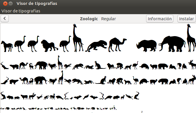
To install a source it is only needed to open it with the typographic viewer of our operating system  and click on Install.

Zoo_01

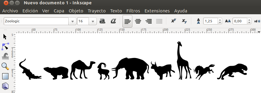
Once installed it will be shown as part of the available fonts in Inkscape. Add text and, for example, if we write “ABCDEFGHI”, something like this will appear:

Zoo_02

We will transform these characters into single images in two simple steps:

  • Path/Object to Path: transform the character into image.
  • Object/Ungroup: create a single image for each character.

Then we have just to select each of them and save one by one as single file by “File/New”, assigning to any single document a size similar to the image ones. Cut and paste the image into this new document (for example the first, the caiman) and by “Object/Align and distribute” align it in the centre. Save it with a name easy to be identified (Caiman.svg). Done.

To have a different symbol when selected, fill the image with yellow colour and “Save as” with the same name but adding at the end “_sel”.

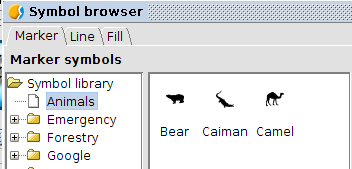
This action can be repeated to as many symbols we want to load. From now on, we only need to use the gvSIG symbol loader in order to have our new symbols library available in gvSIG.

Animals

Posted in english, gvSIG Desktop | 4 Comments

gvSIG 2.0: Gráficas I

Ya está disponible una nueva extensión de gvSIG 2.0 que nos permite trabajar con uno de los documentos más solicitados por la comunidad de usuarios: las gráficas. Las gráficas aumentan las posibilidades del usuarios de gvSIG de representar y analizar los datos, complementando la información proporcionada por los mapas.

Las gráficas tienen multitud de utilidades y, sin duda, son una forma sencilla y visual de comparar entidades, distribuciones, tendencias, etc.

Iniciamos con este post una nueva serie que permita conocer las posibilidades que gvSIG comienza a darnos para trabajar con gráficas.

Para instalar esta nueva funcionalidad seguiremos el procedimiento habitual, abrir el Administrador de complementos, seleccionar la opción de instalación desde URL, elegir el servidor http://downloads.gvsig.org/download/gvsig-desktop/ (en breve estará disponible también en los demás repositorios de gvSIG) y marcar para instalar el paquete Document: charts.

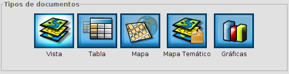
Una vez instalado, cuando reiniciemos nuestro gvSIG para ver reflejados los cambios, nos encontraremos con que disponemos de un nuevo tipo de documento.Gráficas_01

Para poder crear nuestra primera gráfica debemos tener alguna tabla disponible en nuestro proyecto de gvSIG, ya sea una tabla de atributos de una capa o una tabla al uso.

Vamos a hacer nuestra primera gráfica a partir de una tabla que contiene información de población de los países del mundo. Queremos hacer la gráfica sólo de los países de América del Sur, por lo que seleccionaremos estos antes de proceder a crearla.

Seleccionando el tipo de documento “Gráficas” y pulsando “Nuevo” ya tendremos el marco de trabajo de nuestra gráfica creada. Ahora simplemente nos falta indicar sus propiedades para poder visualizarla.Gráficas_02

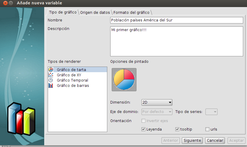
Pulsamos el botón de añadir (botón representado con un “+”) y accedemos a la configuración del gráfico. Vemos que por defecto la extensión nos permite elegir entre 4 tipos de gráficos: de tarta, de XY, temporal o de barras.

En este caso vamos a hacer un gráfico de tarta.Gráficas_03

En la siguiente pestaña “Origen de datos” seleccionamos la tabla y los campos de datos que se utilizarán para el gráfico. En nuestro caso como Etiquetas utilizaremos el campo NAME (que contiene el nombre de los países) y para los valores numéricos el campo POP2005 (que tiene información de la población de estos países en 2005). Activamos la pestaña “Usar sólo campos seleccionados”.Gráficas_04

En la última pestaña vamos a poder definir el “Formato del gráfico” seleccionando propiedades como el color de fondo, contorno o tamaño.Gráficas_05

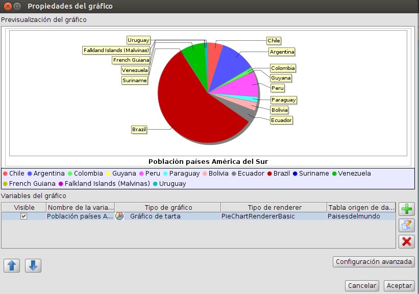
Todo listo, pulsamos “Aceptar” y ya veremos nuestro primer gráfico.Gráficas_06

Por cierto, un mismo documento puede estar compuesto de distintas gráficas, pero eso lo veremos en un siguiente post.

Por último os dejamos un par de vídeos que muestran la instalación de la extensión y los pasos seguidos para crear nuestro primer gráfico.

Nota: Si eres usuario de Windows, recuerda que para poder instalar cualquier extensión debes ejecutar gvSIG como administrador.

Posted in gvSIG Desktop, spanish | Tagged | 1 Comment

gvSIG 2.0: Thematic Maps I

Two available extensions, derived by the gvSIG Batoví project, add very interesting functions for gvSIG 2.0 users.

These two extensions are available through the add-ons manager as:

  • Thematic Maps generator
  • Thematic Maps viewer document

By using both of them it will be possible to work with a new type of document so called “Thematic Map”.

“Thematic Maps” are, in truth, a new type of View offering to the user basic options of querying. The Project gvSIG Batoví aimed originally to provide students, from primary and secondary school, with a tool to easily share maps, without the complex tools available in the gvSIG interface. They can be also a nice base to produce cartographic viewers.

See how it is possible to produce  “Thematic maps” from any “View” and convert this “Thematic Map” in a package that can be installed from any gvSIG (through the add-ons manager). In such a way we can package a  “View” with its own legends, layers, labels and …and distribute to other gvSIG users.

For sure the best way to share information is the Spatial Data Infrastructures, but at small scale and for an easy sharing, “Thematic maps” can represent an interesting tool.

In this video, how to install the application is detailed:

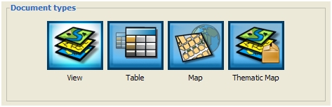
When gvSIG restarts, a new document type appears.

Thematic_Map_menu

In this first post, we will see how to create a “thematic map” from a “View”.

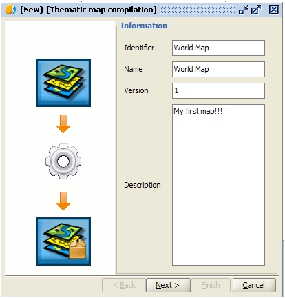
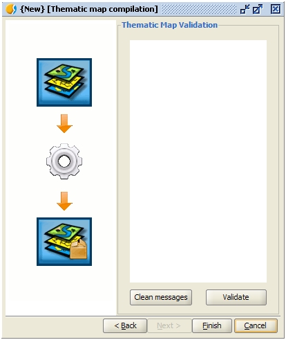
Create a first thematic map from a  “View” with some loaded layers and customized. It is as simple as from our own “View” go to “Thematic Map” and select “Crete from View”. A new window appears where it will be possible to add the characteristics of our map.

 TM_compilation1

Press on “Next” and check that everything is fine. If any of the previous fields has not been filled, a warning appears, even if it is just for information since the procedure continues allowing users to create the “thematic map”.

Description field can be also used to provide information about use of specific symbols libraries in order that, users sharing this thematic map, know that they have to install that library to be able to correctly visualize the map.

 TM_compilation2

Press on “Finish” and  gvSIG automatically creates the new document:

Tematico_04

In the next post we will show how to create packages and share “thematic maps” with other users.

Posted in english, gvSIG Desktop, opinion, training | 3 Comments

gvSIG 2.0: OpenStreetMap, añadiendo nuevos servidores

Una de las pequeñas grandes mejoras que ha presentado gvSIG 2.0 es, en mi opinión, el acceso a la excelente fuente de datos que es OpenStreetMap. La extensión, liberada recientemente, se puede instalar facilmente a través del administrador de complementos de gvSIG (a través de URL seleccionando el servidor http://downloads.gvsig.org/download/gvsig-desktop/ y el paquete Formats: OpenStreetMap raster tiles support).

Como se comentaba en un post anterior, nos va a permitir acceder a las capas de Map Quest, Map Quest Open Aerial, Open cycle Map y Mapnik. gvSIG_OSM_00Una funcionalidad interesante que presenta esta extensión es que podemos añadir nuevos servidores.

Para ello simplemente debemos rellenar los datos del nuevo servidor en la ventana de Añadir capa/OSM.

Veamos un ejemplo añadiendo Terrain uno de los servicios de tiles de Stamen, de Estados Unidos, todos ellos de un excelente diseño.

  • Nombre. Podemos poner lo que queramos, un nombre que nos permita identificar el servidor.
  • URL. La URL del servidor: http://a.tile.stamen.com/terrain
  • Niveles. En este caso son: 17
  • Formato. En este caso es: jpg

Quedaría algo similar a la siguiente imagen:OSM_02Bastaría pulsar el botón de “Añadir servidor” para que pasará a formar parte de nuestro catálogo de servidores.OSM_01De todos los que ofrece Stamen, el que personalmente más me gusta es el que denominan Water Color. Vamos a añadirlo:

Ya sólo nos queda pulsar en “Añadir servidor” y se agregaría al conjunto de servidores disponibles.

Podéis probar a visualizarlo. Tened en cuenta que estos servidores, al contrario de los 4 que vienen por defecto, no todos ofrecen información de todo el mundo. En los casos que Stamen no tiene cobertura global, podéis hacer zoom a una ciudad de Estados Unidos y comprobar como se muestra la nueva información.
OSM_final

Posted in gvSIG Desktop, spanish | Tagged | 10 Comments

gvSIG 2.0: Teselas de OpenStreetMap

La versión 2.0 de gvSIG mejora el acceso ráster incorporando la posibilidad de teselar las fuentes de este tipo de dato, locales o remotas. El resultado es que las capas ráster se cargan sobre la vista de gvSIG en forma de pequeñas porciones o teselas que permite un renderizado progresivo de la capa. Las capas se dividen en niveles preestablecidos de distintas resoluciones y se generan estas teselas para cada nivel en tiempo de ejecución, es decir a medida que se van haciendo peticiones (zooms) de nuevas zonas se van generando las teselas o tiles.

Pero la mayor ventaja de este sistema es que podemos guardar en una caché todos los tiles. De esta forma, la información que se descarga desde los servidores no tiene que volver a pedirse una vez ya se ha hecho, ya que las siguientes peticiones se sirven desde los datos cacheados, con la consiguiente mejora de rendimiento.

De esta forma, la incorporación de nuevas fuentes de datos con este sistema de pirámides de resolución es fácil. Debido a esta posibilidad ha sido relativamente sencilla el desarrollo de un nuevo plugin para el acceso a las capas tileadas de servidores de OpenStreetMap, ya que, como es sabido, estos servidores sirven los datos de esta forma y es totalmente compatible con el sistema de caché incorporado en gvSIG.

Este plugin tiene un acceso básico a las capas de OpenStreetMap para visualización. Por defecto vienen configurado cuatro servidores que sirven las capas de Map Quest, Map Quest Open Aerial, Open cycle Map y Mapnik. En la propia interfaz de “Añadir capa” es posible agregar nuevos servidores, por lo que no nos limita a lo que viene preconfigurado. La interfaz para hacerlo es bastante intuitiva y requiere poca explicación. En mi opinión, este es un ejemplo de como, con poco esfuerzo se pueden aprovechar las posibilidades que de base ofrece gvSIG 2.0 para desarrollar funcionalidad.

Un problema que se presenta gvSIG con las capas de tiles de OSM es la proyección. Estas se sirven en EPSG:3785 y lamentablemente gvSIG no trae configurado de base esta proyección. Es posible crearla manualmente teniendo la cadena WKT, pero resulta algo engorroso. En este caso el plugin lo hará por nosotros. Cada vez que se arranca comprobará si existe este EPSG en la base de datos de gvSIG y si no está la creará como proyección de usuario. De esta forma ya podremos poner la vista en esta proyección para cargar la cartografía.

Otro inconveniente que podemos encontrarnos es que una vez la información está en la caché no se actualiza y si la información cambia en el servidor nosotros seguiremos cargando datos antiguos. Esto no es un problema para capas locales pero para capas remotas, como es el caso de OSM, pues si lo es. Esperemos poder disponer de mejoras que solucionen este problema.

Posted in gvSIG Desktop, spanish | Tagged | 4 Comments

gvSIG 2.0: Data in NetCDF

NetCDF is a data format oriented to scientific data in a multidimensional arrays way. That is, a list of variables with a concrete meaning (pressure, temperature, position…). It’s commonly said that it’s a data container of any type and auto-descriptive. It means that its contents is described in its header.

As generic container it has the advantage of storing raster as well as vector data, and they can be specified for different moments over time. It’s useful for storing on site data that are obtained from sensors where the information collection is periodic and the collected data are varied.

Two plugins have been developed for gvSIG 2.0, that offer support for NetCDF. Its integration in gvSIG has been made from the point of view of the same application, separating the support in two different data providers: raster and vector. It’s because its graphical representation in gvSIG is totally different. With the incorporation of this format, gvSIG can load and export data with time information.

But the time information requires a special treatment in any Geographic Information System, now that the user should be able to filter the information to be shown in a specific moment or in a temporary interval. Besides the user should be able to process the data taking the moment into account or even to be able to make animations throughout time. In this sense gvSIG has improved in an important way, because it incorporates this functionality (data filter by time and short animations). At this moment this tool has to be improved to make geoprocessing on layers with time information, besides integrating time support on the raster part. We hope to improve this issues in the future versions, although these plugins are available now.

Posted in gvSIG Desktop, opinion, spanish | 1 Comment

gvSIG 2.0: Biblioteca de símbolos “Emergency”

Uno de los ámbitos en los que gvSIG se está utilizando cada vez más es en el de gestión de emergencias, tanto a nivel urbano como de catástrofes naturales. Sin duda, es más que significativo el aporte que el análisis espacial puede suponer para la gestión de emergencias y campos relacionados como el análisis delictual.

Orientada a estos usuarios hemos realizado una nueva biblioteca de símbolos. Como es habitual disponible desde el “Administrador de complementos”.

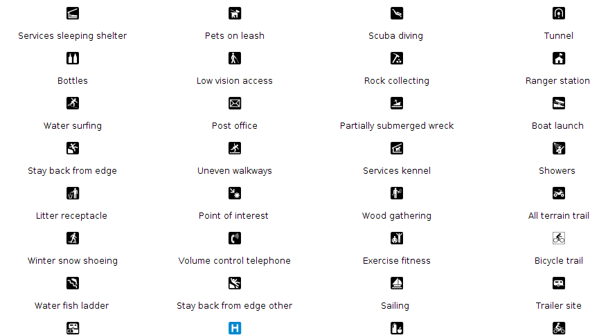
Para los símbolos puntuales (marcadores) hemos partido de un conjunto de símbolos denominado “EMS.The Emergency Mapping Symbology”, realizado por el Departamento de Recursos Naturales de Canadá  que tal y como indican es de libre uso. La forma de importarlos ha sido la habitual, descrita en este post.

Como en casos anteriores hemos utilizado pyRenamer -una herramienta de renombrado masivo de archivos-, ya que el nombre que gvSIG da a cada símbolo es el nombre del fichero. El objetivo del renombrado es facilitar la identificación de símbolos.EMS_01Estos símbolos están diseñados para utilizarse con un tamaño de 32 píxeles -con el objetivo de resaltar su importancia en el mapa- por lo que los hemos importado a ese tamaño. Reduciéndolo a tamaños inferiores también se visualizan correctamente.

Mediante GIMP hemos generado los distintos símbolos de selección. En este caso, al haber símbolos con tonalidades de amarillo, hemos decidido que los símbolos de selección se representen en escala de grises. Con la opción de GIMP Imagen/Modo/Escala de grises hemos convertido los símbolos a escala de grises, añadiendo “_sel” al nombre del fichero para que gvSIG lo interprete automáticamente como símbolo de selección.

Además de símbolos puntuales, queríamos que esta biblioteca contuviera un conjunto de símbolos de líneas y relleno útiles para los mapas de emergencias, delitos,etc.

Hemos generado tanto símbolos lineales:EMS_02Como símbolos de relleno, inspirados en el documento Biosecurity Emergency Management – Mapping Symbology:EMS_03Ya sólo nos queda crear el paquete tal y como explicamos en este post.

Este paquete lo tenéis disponible desde el administrador de complementos (seleccionando la URL http://downloads.gvsig.org/download/gvsig-desktop/ y buscando por “Tipos/symbols”)o directamente descargándolo desde aquí.

Posted in gvSIG Desktop, spanish | Tagged | 3 Comments

gvSIG 2.0: Scripting, exploit your gvSIG (III): Generate a polygon from a course

Some time ago a friend of the project, Gustavo Agüero, published a post on his blog in which he explained how gvSIG generate a polygon from a bearing (or route or course). We found a very interesting exercise and with its help we implemented a script to undertake the same steps in gvSIG 2.0. The result is explained in this post.

We want to clarify that all the merit of this exercise is to Gustavo and the errors are because of our ignorance and for not properly follow his instructions. If you see some error, please, comment it and we will correct it 😉

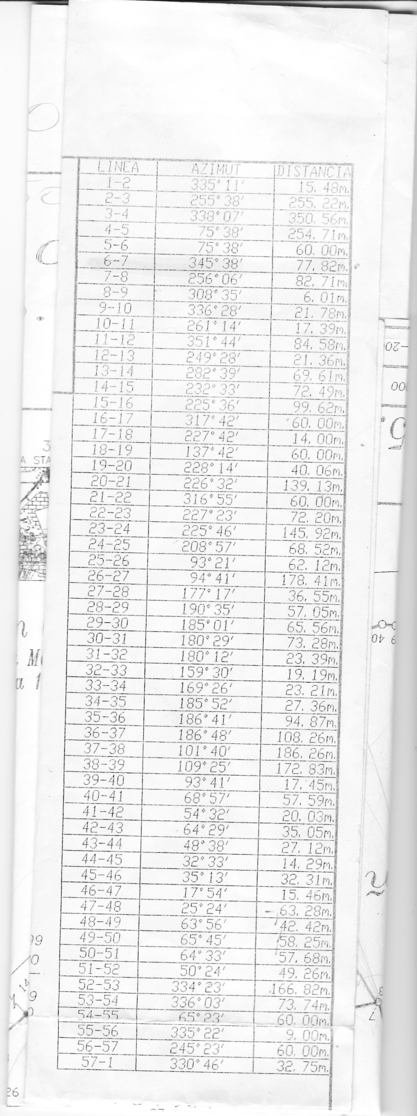
We start with a bearing or course that presents the data to the following structure LINE, AZIMUT, DISTANCE, being AZIMUT the angle direction in the sense counted clockwise from the geographic north (download rumbo.jpg).

The first thing to do is to save this file to a format that would be able to read from a script, this file we have created is a csv file that we named rumbo.csv (download rumbo.csv).

Once we have our file we have to think what we need to get its content into a shapefile. Obviously we’ll need a shapefile where to save the results and we’ll need to create the features to represent the data for including them on the shapefile. To create these features we’ll need to transform the polar coordinates (azimuth, distance) in rectangular coordinates (X, Y).

Some comments on that: Gustavo in his post recommend to make a representation of the data. This was very helpful to us.

In the script we will create a LINE shapefile and another one for POLYGONS. In the LINE type, we will keep heading data, data from coordinates transformation, and the resulting coordinates. In the POLYGONS shapefile will keep an identifier of the feature and a text field.

We start from a desktop gvSIG 2.0 (in my case I’ve used is build 2060 RC1) with the latest version of the scripting extension installed (currently the number 36).

Once we open the script editor (menu bar Tools / Scripting / Scripting Composer) we create a new script and start to write our script.

The first thing we’re going to do is to create the output layers using the function createShape from the gvsig module. The syntax of this function tells us that you need a data definition for the features, a route that is the place where to store the shapefile we are acreating, the projection of the shapefile, and the type of geometry that will contain. The definition of the data will be created using the function createSchema from the same gvsig module.

The source code, including comment would be:

import gvsig
import geom

def main():

'''
Create a polygon layer with the following data model:
    - 'ID', Integer
    - 'OBSERVACIONES', string
    - 'GEOMETRY', Geometry

Create a line layer with the following data model:
    - "ID", Integer
    - "LINEA", string
    - "GRADOS", long
    - "MINUTOS",long
    - "DISTANCIA", double
    - "RADIAN", double
    - "X", double
    - "Y", double
    - "GEOMETRY", Geometry            
'''

#Set up the projection, it is the same for both layers
CRS="EPSG:32617"

#Create the object that represent the data model for the polygonal shapefile
schema_poligonos = gvsig.createSchema() 

#Insert the filed from the data model
schema_poligonos.append('ID','INTEGER', size=7, default=0) 
schema_poligonos.append('OBSERVACIONES','STRING', size=200, default='Sin modificar') 
schema_poligonos.append('GEOMETRY', 'GEOMETRY')

#Set up the layer path. Remember changing it!!!
ruta='/tmp/rumbo-poligonos.shp'

#Create the shapefile
shape_poligonos = gvsig.createShape(
        schema_poligonos, 
        ruta,
        CRS=CRS,
        geometryType=geom.SURFACE
    )

#Create the line shapefile

#Create the object that represent the data model for the line shapefile
schema_lineas = gvsig.createSchema() 

#Insert the field from the data model
schema_lineas.append('ID','INTEGER', size=7, default=0) 
schema_lineas.append('LINEA','STRING',size=50,default='')
schema_lineas.append('GRADOS','LONG', size=7, default=0) 
schema_lineas.append('MINUTOS','LONG', size=7, default=0)
schema_lineas.append('SEGUNDOS','LONG', size=7, default=0) 
schema_lineas.append('DISTANCIA','DOUBLE', size=20, default=0.0, precision=6) 
schema_lineas.append('RADIAN','DOUBLE', size=20, default=0.0, precision=6) 
schema_lineas.append('X','DOUBLE', size=20, default=0.0, precision=6) 
schema_lineas.append('Y','DOUBLE', size=20, default=0.0, precision=6) 
schema_lineas.append('GEOMETRY', 'GEOMETRY')

#Set up the layer path. Remember changing it!!
ruta='/tmp/rumbo-lineas.shp'

#Create the shapefile
shape_line = gvsig.createShape(
    schema_lineas, 
    ruta,
    CRS=CRS,
    geometryType=geom.MULTILINE
)

Ok, we already have our output layers, now we are going to see how to get the data from csv file we created. Python has a module that allows csv csv file handling very comfortable ( python csv ). The source code for reading the csv file would be:

import csv
import os.path

#Set up the layer path for the CSV file. Remember changing it!!!
csv_file = '/tmp/rumbo.csv'

#Check that the file exists on the provided path
if not os.path.exists(csv_file):
  print "Error, el archivo no existe"
  return

#Open the file on read only mode
input = open(csv_file,'r')

#Create a reader object from the CSV module
reader = csv.reader(input)

#Read the file
for row in reader:
    #Print the line
    print ', '.join(row)

We already know how to create shapefiles and read csv files, the next step would be to create the features, so we must transform the polar coordinates to rectangular and it is at this point that for me things get a little dark so forgive the errors that you can find.
To make the coordinate transformation we’ll convert the decimal angle in radian angle. Gustavo in his post how to generate a polygonal (in Spanish) between the files to download you can find a PDF that provides an explanation of the calculations he made, if anybody has doubts I recommend to read it. I only want to clarify that we ‘ll use the python module python math to use math functions sine and cosine, needed to perform the transformation. In addition, our course uses relative coordinates, so we need a starting point and the code to calculate the new coordinates from the above ones. Our starting point is ( X= 361820.959424, Y = 1107908.627000). The source code would be:

"""
Convert decimal degrees, minutes, seconds to radian
"""
import math
#Define the “pi” value
PI = 3.1415926

x_ant = 361820.959424
y_ant = 1107908.627000

#Apply the equation and obtain the angle in radians
angulo = (degrees+(minutes/60.0)+(seconds/3600.0))*PI/180.0

#Convert the polar coordinates into rectangular ones

x_new = radio * math.sin(angulo)
y_new = radio * math.cos(angulo)

#Add relative coordinates values to get the next coordinate
x = x_new + x_ant
y = y_new + y_ant

The last piece of our puzzle is to learn how to create the features and their geometries. The layers that we created earlier shape_line and shape_polygons have a method called append that allows us to add the features to the layer. This method accepts a dictionary,
python dict that uses as key fields the ones we defined in the data structure of the layer (defined when we created it). The values are the ones that should have the feature. The geometries will be created using the geometric module geom from the scripting extension, in particular the createGeometry function, that needs the type of geometry to be created and the dimensions of the geometry. The code that we could use is:

geometry_multiline = geom.createGeometry(MULTILINE, D2)

values = dict()
values["ID"] = id #Calculated field for the registered number
values["LINEA"] = linea_id #First data of the course
values["GRADOS"] = grados #decimal degrees from the course
values["MINUTOS"] = minutos #decimal minutes from the course
values["SEGUNDOS"] = segundos #decimal seconds from the course
values["DISTANCIA"] = radio #Distance from the course
values["RADIAN"] = angulo #Radian angle calculated
values["X"] = x #X coordinate calculated
values["Y"] = y #Y coordinate calculated

shape_line.append(values)

At this point we have seen everything needed to get what we want from our original course, we only need to assemble the puzzle and the final result would be this:

Polígono

Polygon generated from the course

The final source code can be downloaded from here .

We hope you enjoy that exercise as much as I do.

See you next time!

Posted in english, gvSIG Desktop, scripting | Leave a comment

gvSIG 2.0: Biblioteca de símbolos “Forestry”

Uno de los ámbitos habituales de uso de los SIG es el forestal. Orientada a esos casos de uso hemos realizado una nueva biblioteca de símbolos. Y como es habitual disponible desde el “Administrador de complementos”.

Veamos como hemos realizado esta biblioteca, de modo que sirva como un nuevo ejemplo a los usuarios para crearse las suyas propias.

Para los símbolos puntuales (marcadores) hemos partido de dos fuentes distintas:

– Por un lado la colección de símbolos utilizada por el NPS (U.S. National Park Service). Una excelente colección de símbolos de dominio público.

– Por otro lado hemos utilizado la fuente Trees & Shrubs realizada por Jim Mossman, también de dominio público.

Para añadir los símbolos de NPS, hemos seguido lo indicado en este post. Para facilitar la identificación de símbolos, hemos utilizado una herramienta de renombrado masivo de archivos, ya que el nombre que gvSIG da a cada símbolo es el nombre del fichero; en nuestro caso hemos utilizado pyRenamer. Mediante Inkscape hemos generado los distintos símbolos de selección (coloreando de amarillo cada símbolo y añadiendo la terminación “_sel” al nombre del fichero).

Todo preparado para utilizar el importador de símbolos de gvSIG. Importamos los símbolos a “Forestry/NPS”. De forma automática se crea la nueva biblioteca con el conjunto de símbolos puntuales importados.foresty_point2

A partir de lo indicado en este otro post generamos los distintos ficheros SVG que representan un conjunto de árboles y arbustos. Utilizamos el importador de símbolos, almacenándolos en Forestry/Trees & Shrubs.Forestry_point1

Además de símbolos puntuales, queríamos que esta biblioteca contuviera un conjunto de símbolos de líneas y de relleno habituales en los mapas forestales.

Hemos generado tanto símbolos lineales:Forestry_lineaComo símbolos de relleno:Forestry_relleno


Ya sólo nos queda crear el paquete tal y como explicamos en este post.

Este paquete lo tenéis disponible desde el administrador de complementos (seleccionando la URL http://downloads.gvsig.org/download/gvsig-desktop/ y buscando por “Tipos/symbols”)o directamente descargándoos el paquete desde aquí.


Posted in gvSIG Desktop, spanish | Tagged | 4 Comments